FUTURES: Urban Growth Modeling at Scale
Anna Petrasova
NCSU GeoForAll Lab
at the
Center for Geospatial Analytics
NC State University
DOI, Open GIS Group, Dec 2nd, 2021
Anna Petrasova
- BS & MS in Geoinformatics, Czech Technical University in Prague
- PhD in Geospatial Analytics, NC State
- Geospatial Research Software Engineer at the Center for Geospatial Analytics, NC State
- GRASS GIS Development Team Member
- GRASS GIS Project Steering Committee Member
- Open Source Geospatial Foundation Charter Member
FUTURES
- developed at Center for Geospatial Analytics (CGA), NC State
- to address the regional-scale environmental impacts of urbanization
- explicitly captures the spatial structure of development
- flexible (in terms of predictors, scenarios)
FUTure Urban-Regional Environment Simulation
FUTURES
- simulates urban growth (undeveloped to developed)
- accounts for location, quantity, and pattern of change
- patch-based land change model
- stochastic
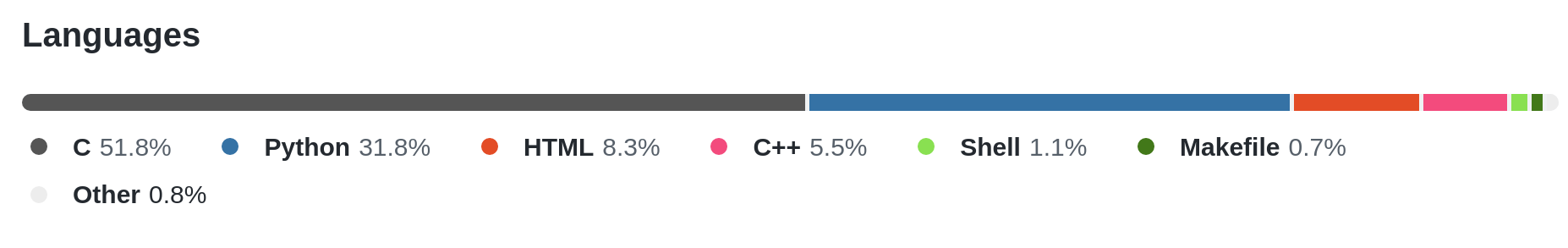
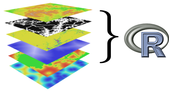
FUTURES software implementation
- open source
- GRASS GIS addon
- set of modules r.futures.*
- written in C and Python
- runs on all platforms
- hosted on GitHub

Why GRASS GIS?
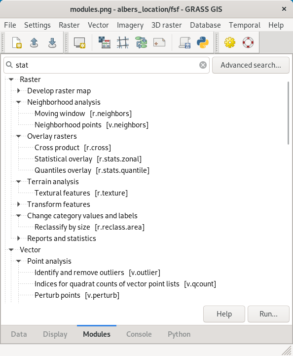
All needed GIS functions at hand
Why GRASS GIS?

Automatically generated CLI and GUI
Why GRASS GIS?
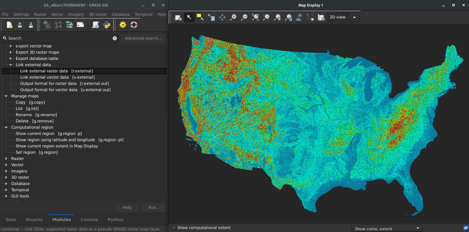
Efficient I/O libraries and processing of large datasets
Why GRASS GIS?
Modular architecture: modules in C/C++ and Python
Why GRASS GIS?
Infrastructure for online manual pages and distribution of binaries
Why GRASS GIS?
Maintained by community and developers
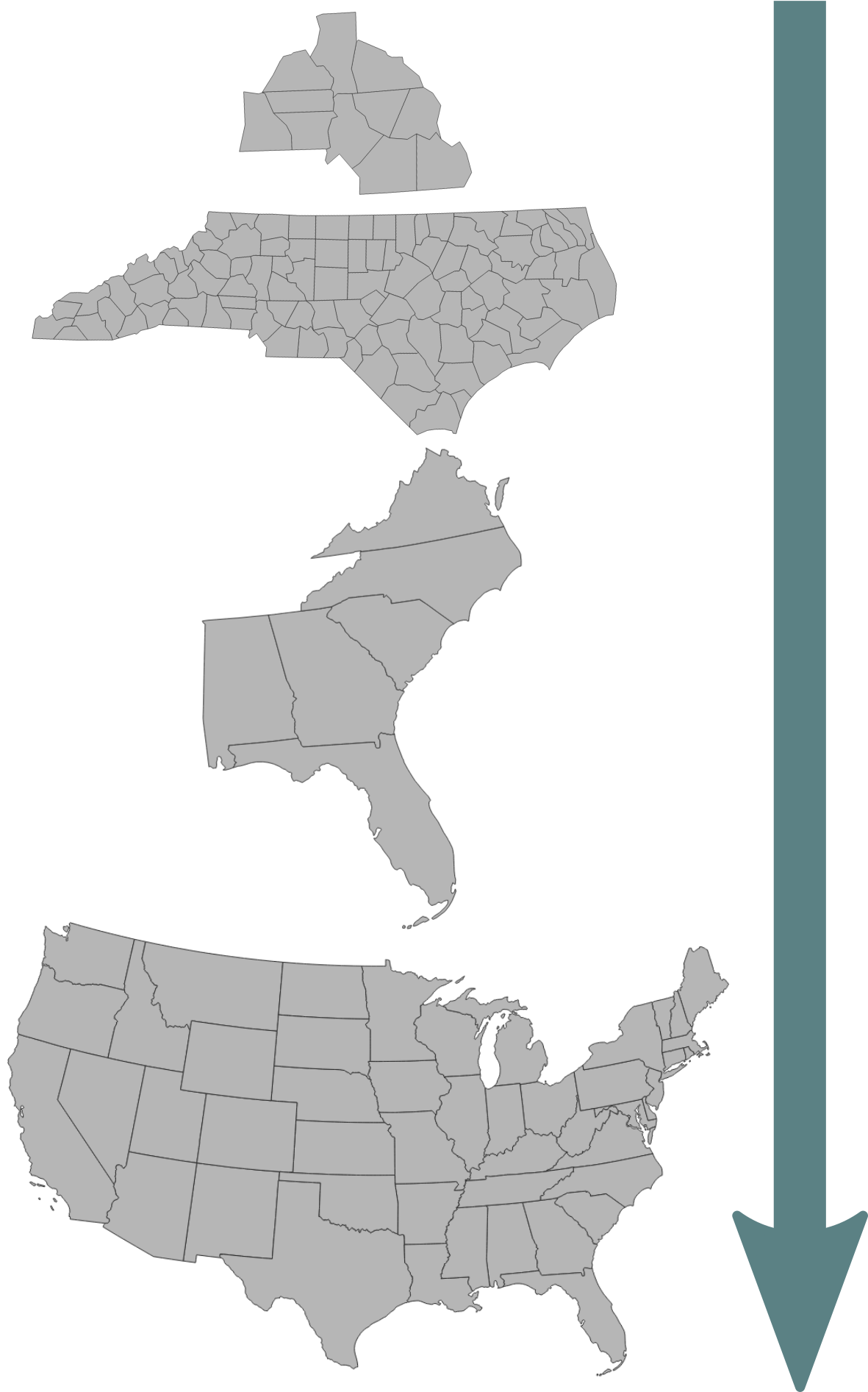
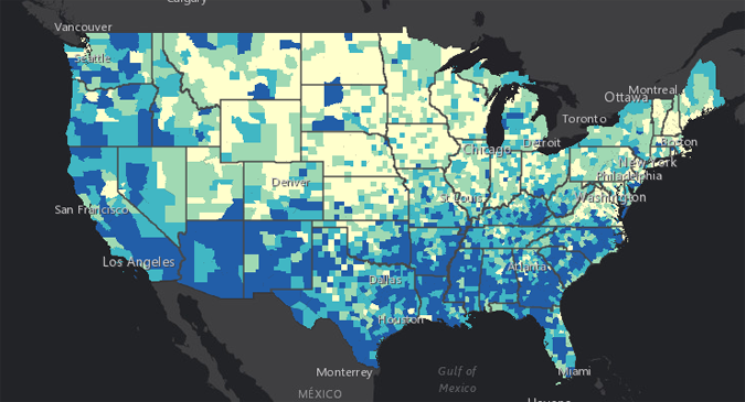
Why CONUS case study?
- previous case studies showed potential to scale up
- available datasets (NLCD, etc.)
- available computing infrastructure
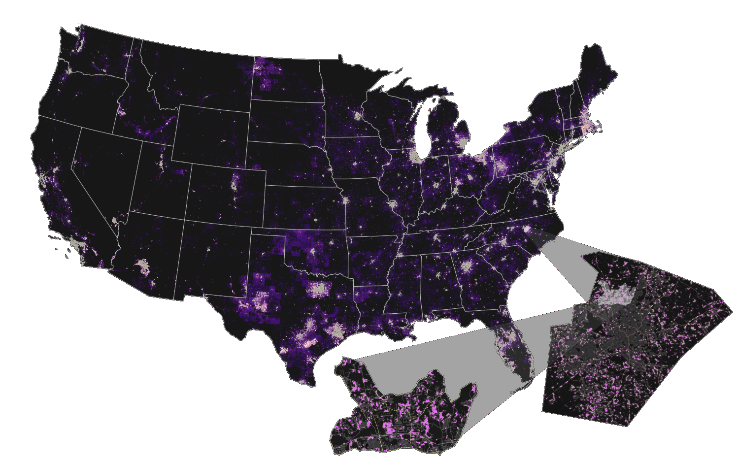
- to provide detailed national urbanization projections
- to study urbanization trends inside and outside of floodplain
16,000,000,000 cells at 30 m resolution
Input datasets: Land cover
NLCD 2001 - 2019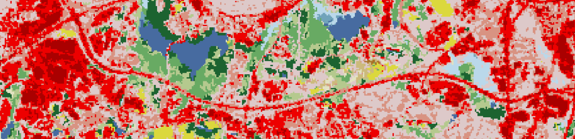 Land cover
 Impervious descriptor
Input datasets: Population
- past population (SEER)
- county level population projections (Hauer et al. 2019)
- shared socioeconomic pathway SSP2 (Middle of the Road)
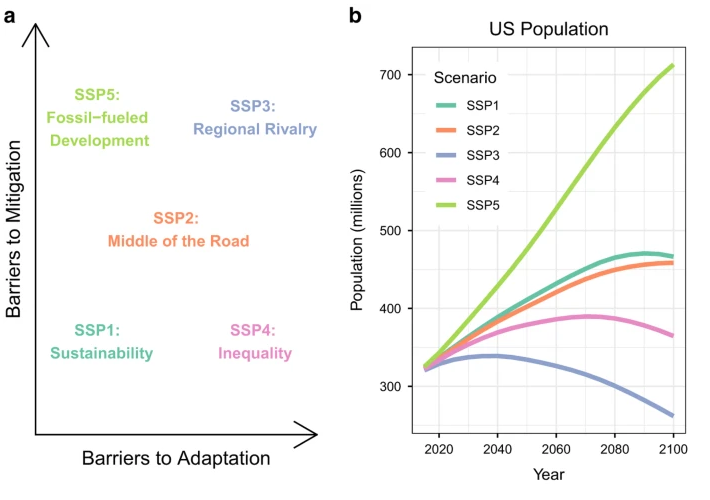
source: Hauer et al 2019
Input datasets
- NED DEM (USGS)
- protected areas (PAD-US by USGS)
- USA National Commodity Crop Productivity Index
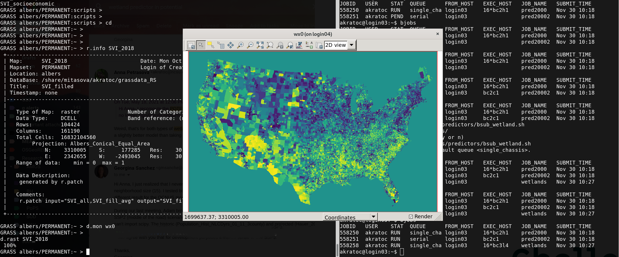
- CDC Social Vulnerability Index
- boundary datasets: counties, metropolitan statistical areas
SVI, source: CDC
FUTURES schema
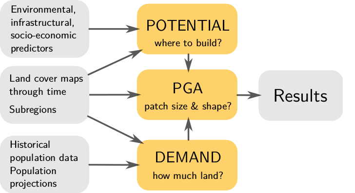
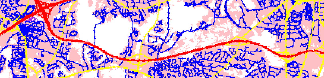
Where to develop?
- Derive predictors (distance to water, roads, forest, SVI, crop index, slope)
- Derive newly developed pixels (raster algebra)
- Sample predictors (2,000,000 points)
- Run logistic regression for different combinations of predictors
- Create development suitability surface
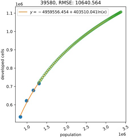
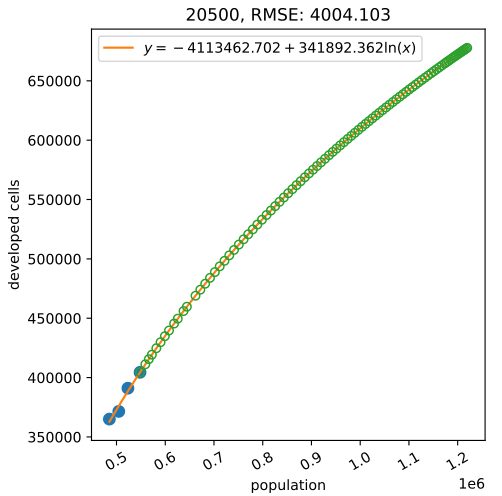
How much land?
Projects land consumption for each year and county
based on NLCD and past and projected population:
Raleigh-Cary Metro Area
 NC
NCWhat is the size and shape?
- Calibrate patch size and compactness from past urban change
- Grow patches in suitable areas until demand met
NCSU Henry2 cluster
- Total nodes online: 933
- Total cores online: 13644 (2021-11-19)
- Python, R, GRASS GIS
*******************************************************************************
*                                                                             *
*               North Carolina State University, Raleigh, NC 27695            *
*                      Office of Information Technology                       *
*                           http://hpc.ncsu.edu/                              *
*                                                                             *
*******************************************************************************
*                                                                             *
*                      Welcome to henry2 Linux cluster                        *
*                                                                             *
*******************************************************************************
*******************************************************************************
*                           WARNING - USER BEWARE                             *
*                                                                             *
*   This is a NC State HPC Production System. Use of this system is subject   *
*   to NC State Computer Use Policy - policies.ncsu.edu/policy/pol-08-00-01   *
*   and the OIT HPC Acceptable Use Policy - hpc.ncsu.edu/About/AUP.php        *
*                                                                             *
*   Share/scratch/tmp-space is NOT being backed-up and files are subject to   *
*   deletion at any time. You use share/scratch/tmp disk space at your own    *
*   risk.                                                                     *
*                                                                             *
*   Security violations, and unauthorized or unlawfull use of this system     *
*   will be prosecuted.                                                       *
*                                                                             *
*******************************************************************************
Parallelization approaches
Most of our tasks are "pleasantly parallel"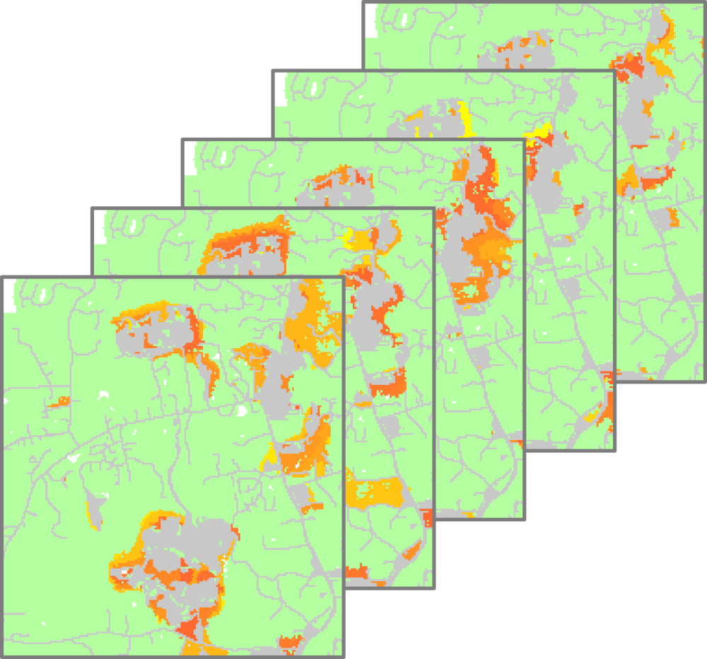
independent computations (stochastic runs)
divide spatial domain (tiles with overlaps, states, counties)
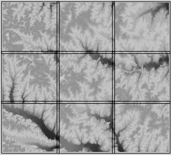
Tiling approach example
Moving window analysis with large window size parallelized using GRASS GIS GridModule:
        grd = GridModule("r.futures.devpressure", width=161200, height=6600, overlap=30, processes=16, **params)
        grd.run()
Tiled raster algebra:
r.mapcalc.tiled "dist_to_forest_log = log(dist_to_forest)" width=161200 height=6600 processes=16
Caveats:
- Doesn't scale across nodes (max 30 cores per node)
- How you do tiling impacts performance
- Overhead can make it slower than without tiling
- Does not work for certain algorithms (e.g. hydrology)
Independent runs
Distribute computing across nodes using MPI (Message Passing Interface standard):jobs.txt
grass --tmp-mapset ~/grassdata/albers/ --exec r.futures.demand subregions=subregion_1 output=file1.csv ...
grass --tmp-mapset ~/grassdata/albers/ --exec r.futures.demand subregions=subregion_2 output=file2.csv ...
grass --tmp-mapset ~/grassdata/albers/ --exec r.futures.demand subregions=subregion_3 output=file3.csv ...
submit.sh
        mpiexec python -m mpi4py -m pynodelauncher myjobs.txt
Caveats:
- Need to know how much memory you need and assign number of cores per node accordingly
- Gets tricky if some processes take much longer than others (looking at you, Texas)
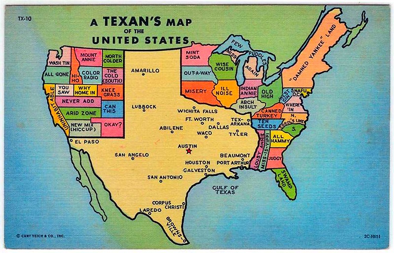
texasproud.com/how-big-is-texas-its-huge
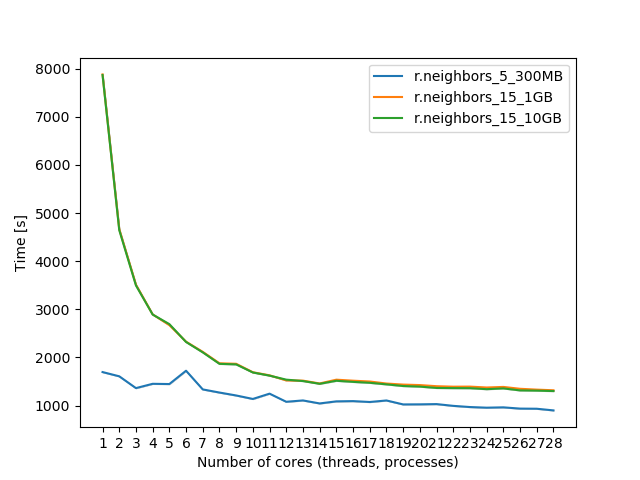
Parallelization using OpenMP
- Implemented on algorithm level (C/C++)
- Shared-memory parallelism (doesn't scale across nodes)
- Convenient for user
- Newly parallelized modules in GRASS GIS thanks to GSoC 2021
Memory handling
- Can't fit entire study area into memory
- Parallelization by states leads to unequal memory consumption
- GRASS GIS segment library: only loads what fits in memory
r.futures.pga ... memory=12000 - example of HPC submission parameters (9 processes per node, 3 nodes, 120GB each)
            #!/bin/bash
            #BSUB -n 27
            #BSUB -R "rusage[mem=120GB]"
            #BSUB -R span[ptile=9]
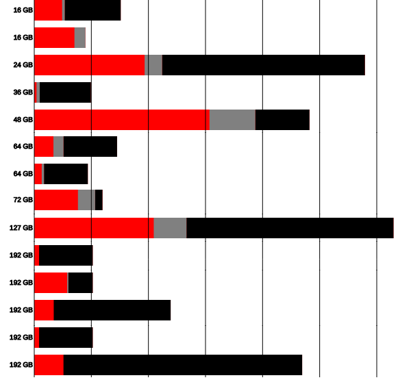
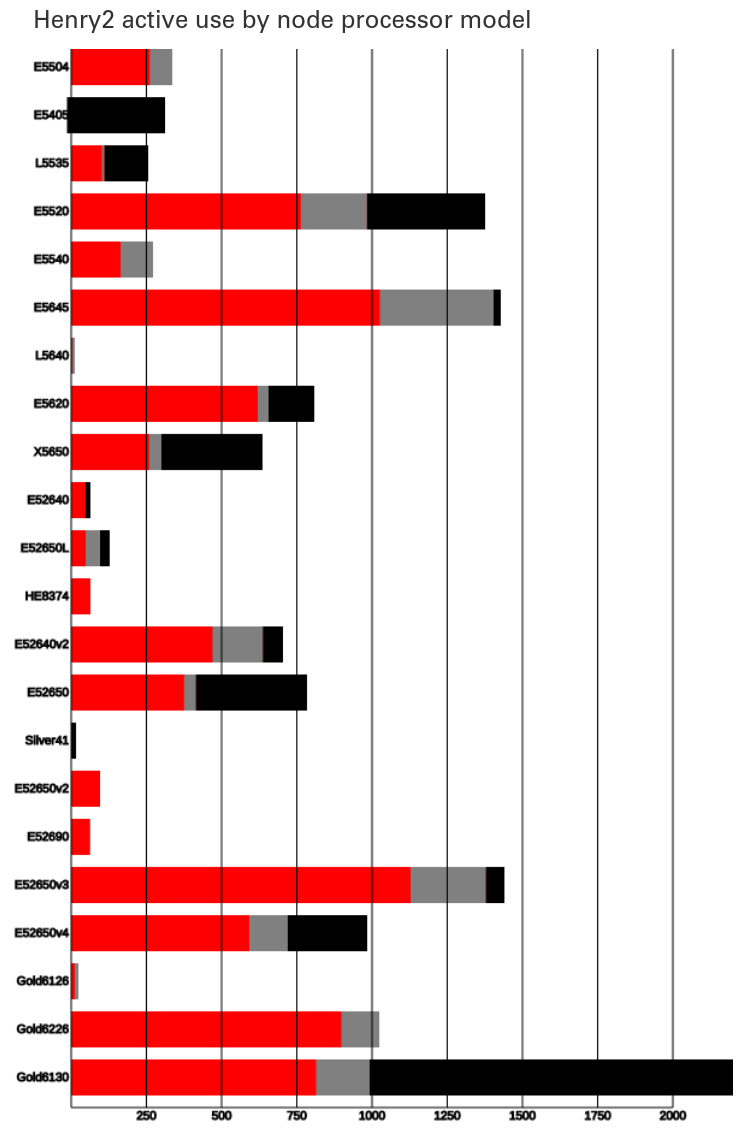
Henry2 nodes by memory (edited)
Challenges
GIS on HPC
Parallelization by states
We needed to respect Metropolitan Statistical Areas boundaries: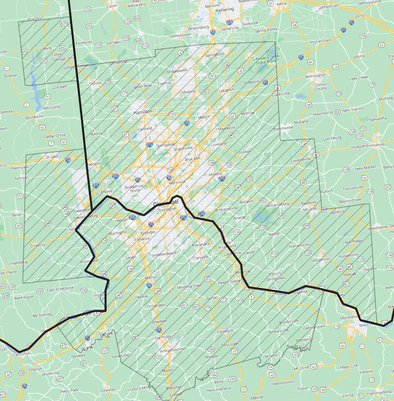
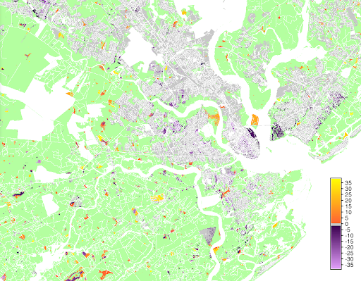
SSP5 scenario

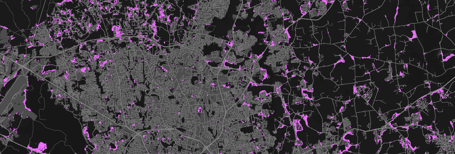
New development by 2100
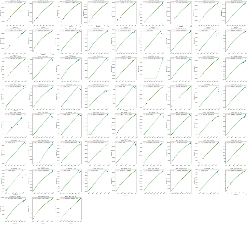
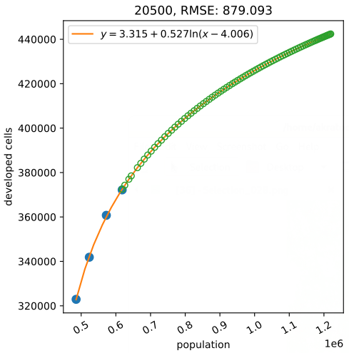
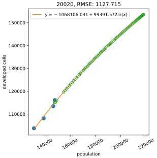
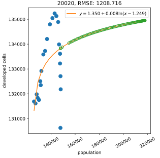
Automatic fitting of densification curves
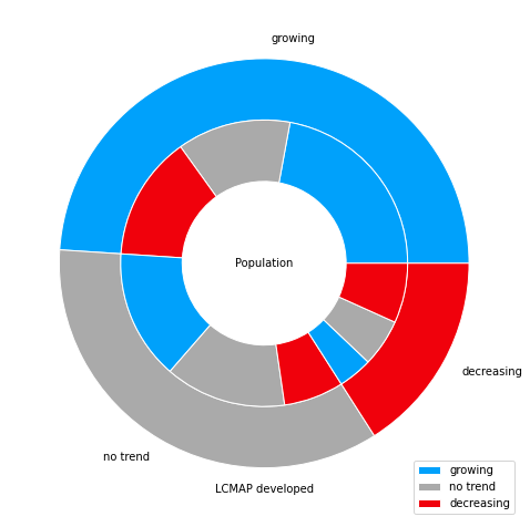
LCMAP or NLCD?
Similar products: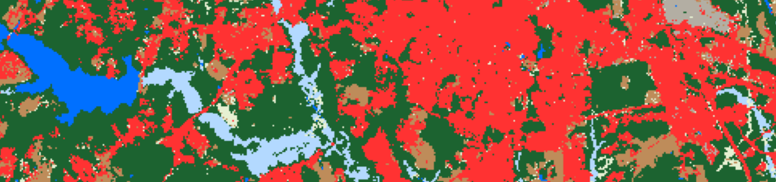 LCMAP: completely automated, 33-year historical period
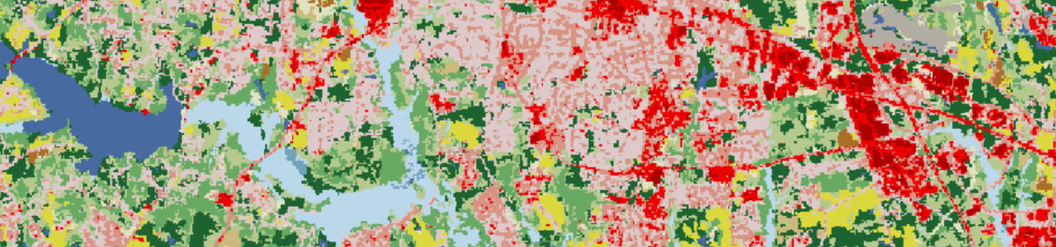 NLCD: higher level of thematic detail
LCMAP: decline in developed area
NLCD vs LCMAP developed area trends

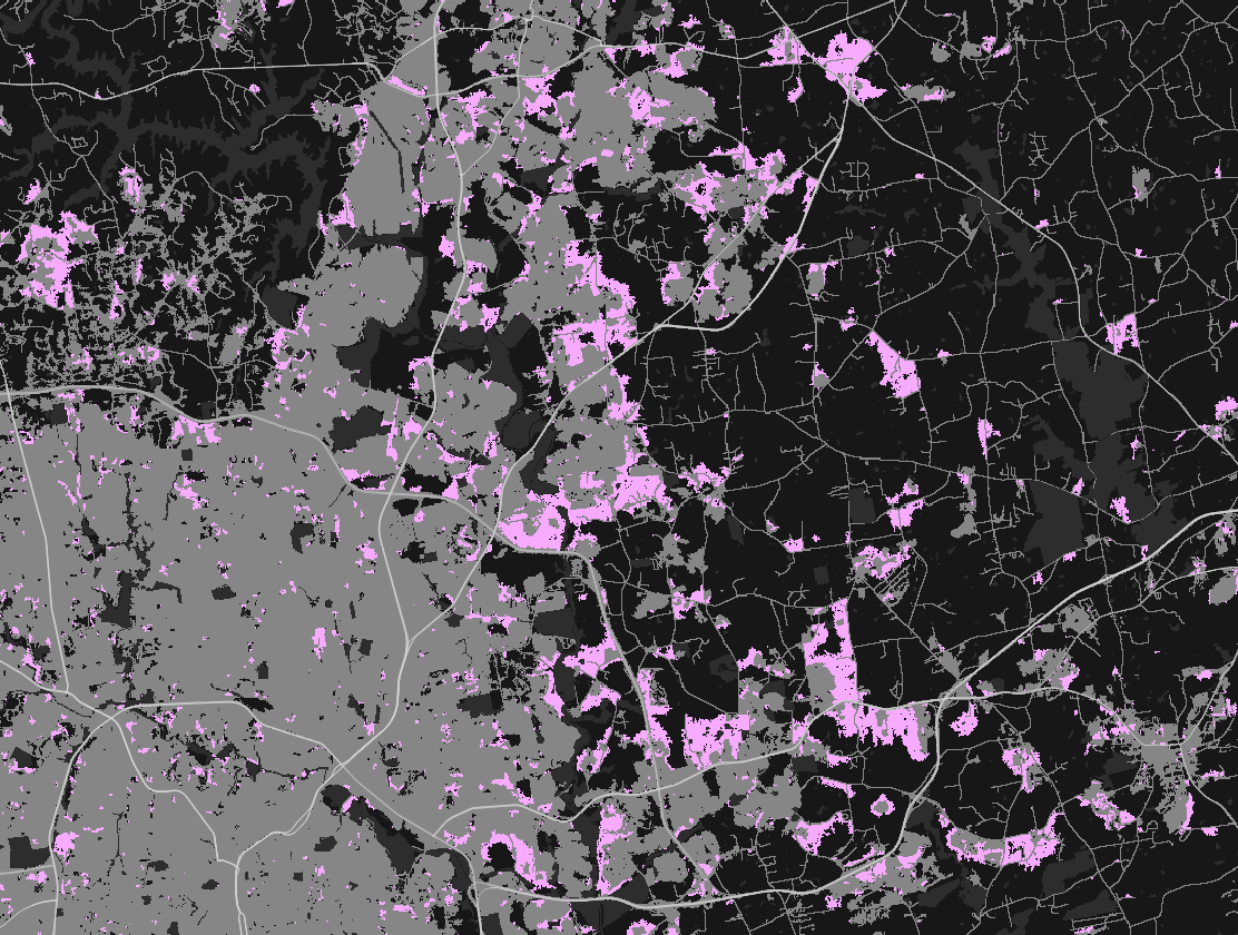
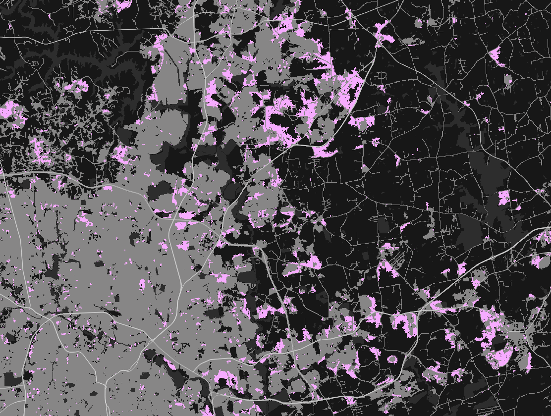
Results
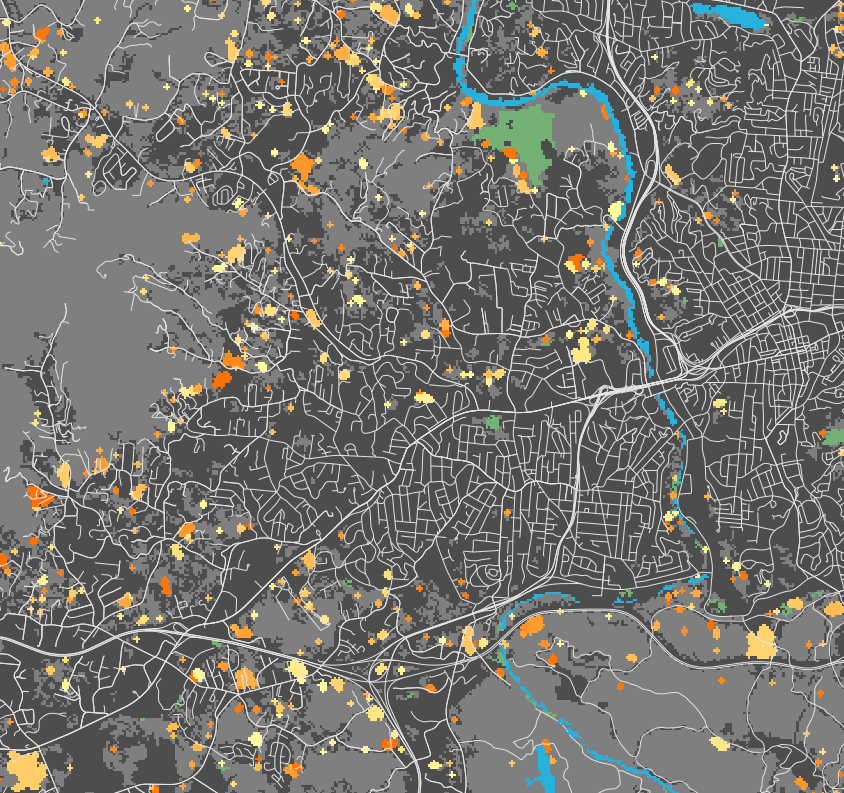
(preliminary)NE Raleigh by 2100
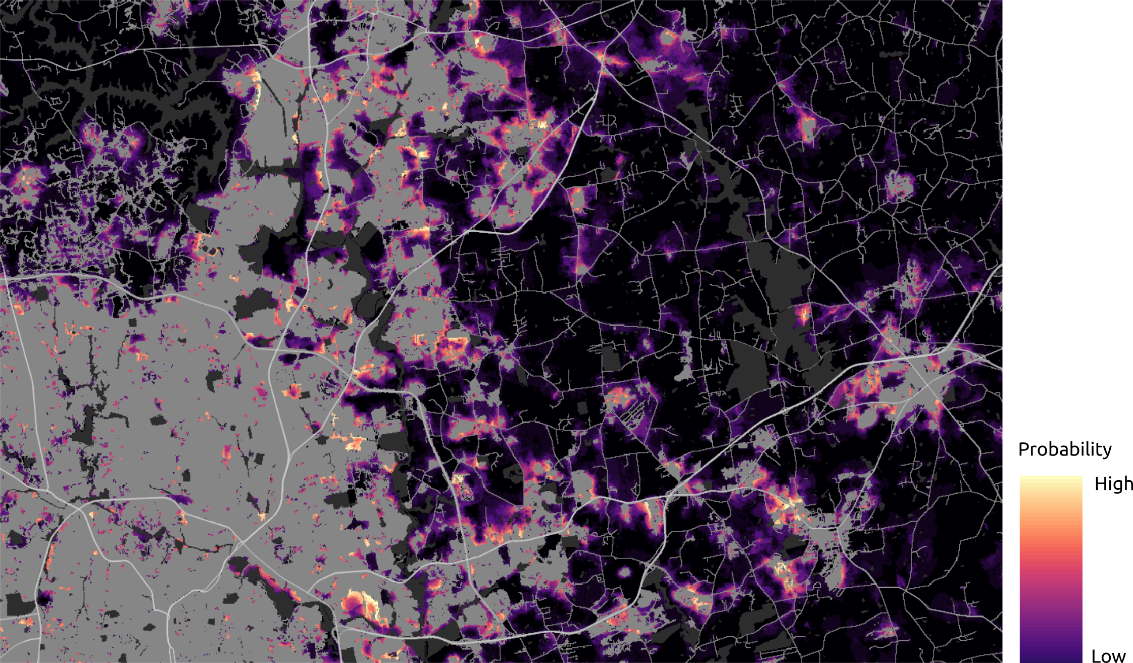
NE Raleigh: probability
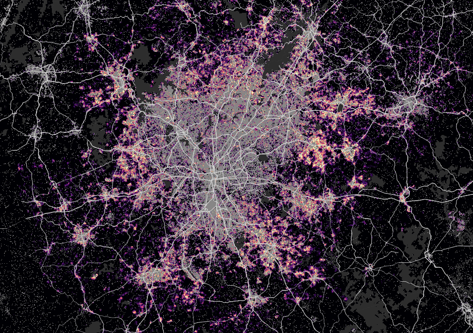
Atlanta
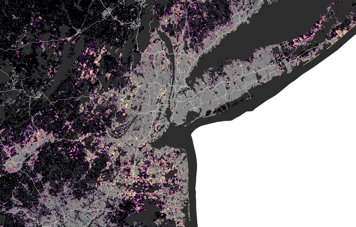
New York
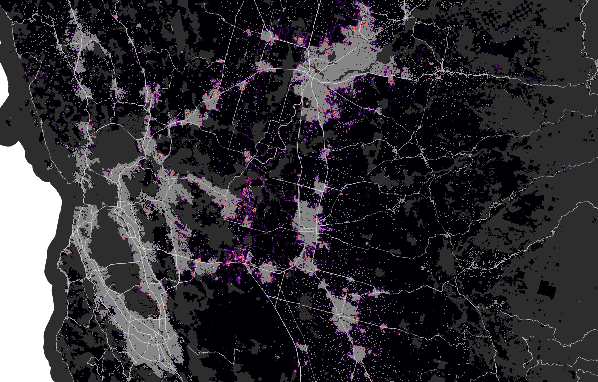
San Francisco
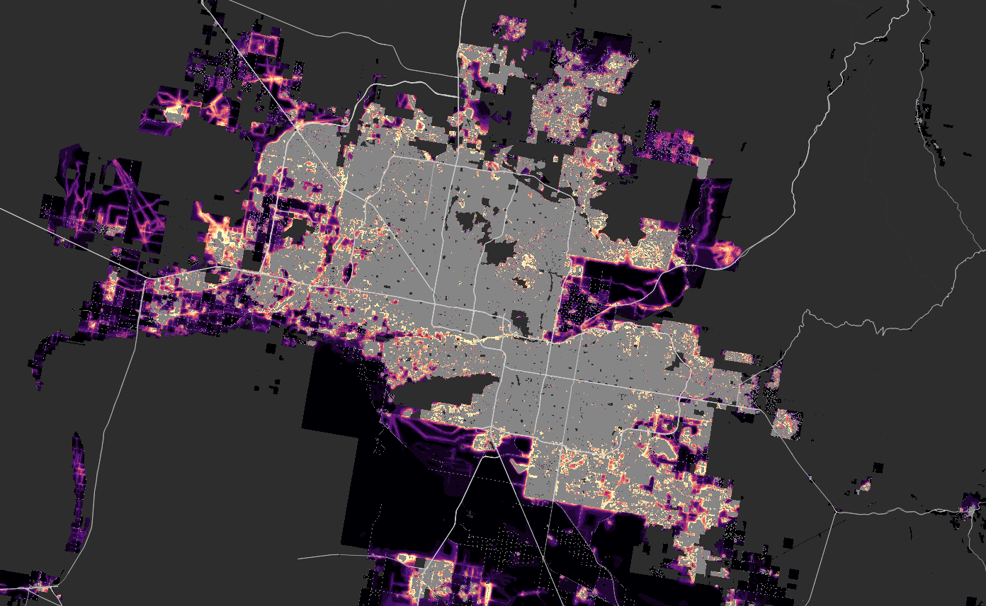
Phoenix
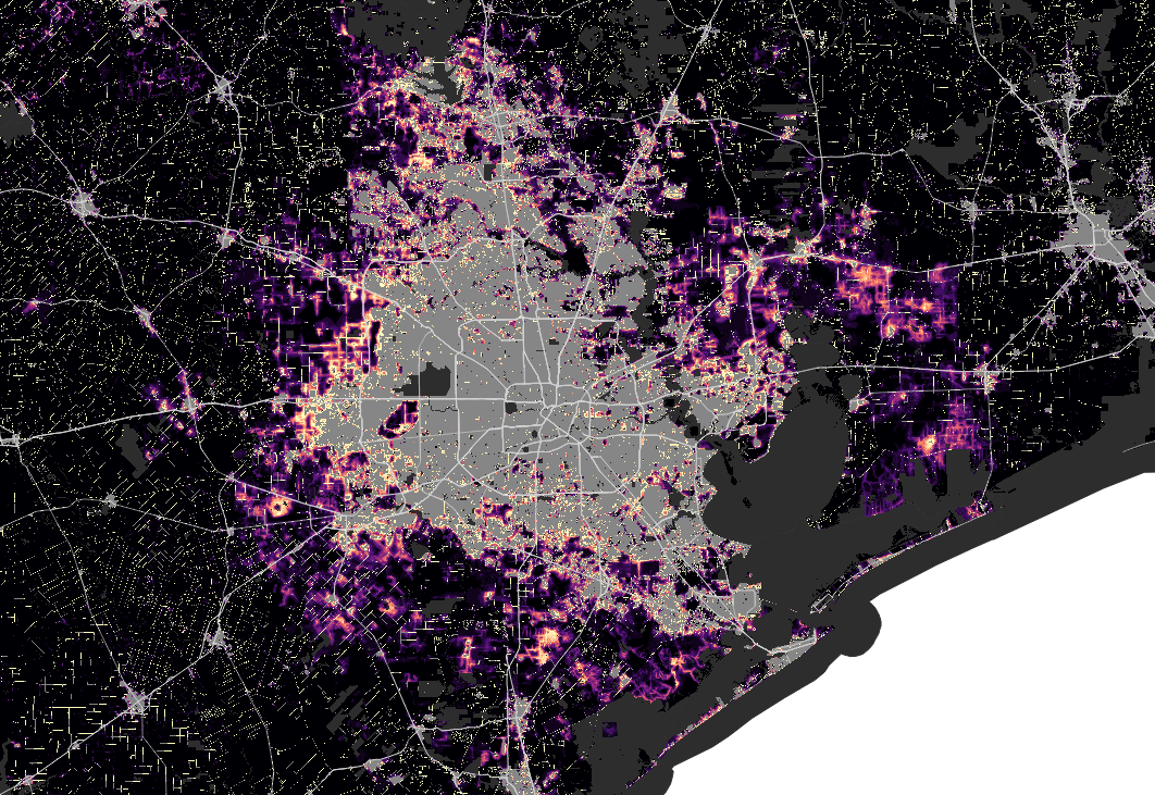
Houston
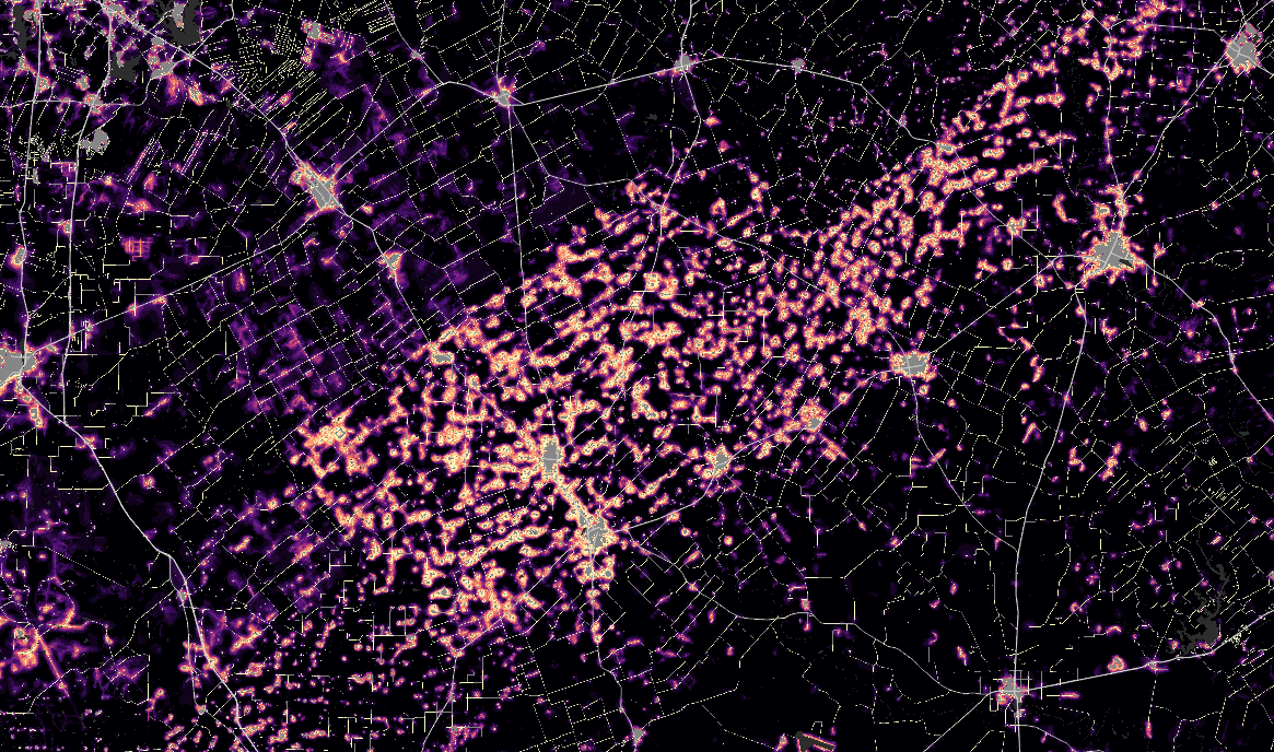
Karnes County, TX
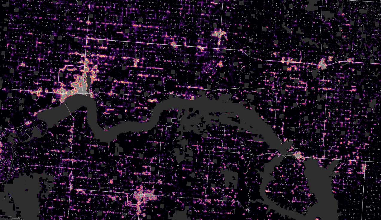
North Dakota
Benchmark examples
- Simple raster algebra
- 30 min without paralellization
- 10 min with tiling approach on 16 cores
- Stratified random sampling
- approx 2 mil points, 30 rasters
- 2.6 hours on 200 cores
- FUTURES patch growing simulation
- 20-30 hours on 27 cores on 3 nodes with 120 GB each
- simultaneosly running jobs with different random seeds
FUTURES v3
Incorporates flood hazard and response (retreat, adaptation) into modeling of future urbanization